NOTE: The benchmark and analysis code are available here.
As a computer architect, I always find an unexplained bandwidth number a bit annoying. While experimenting with the Tensor Memory Accelerator (TMA) on Hopper, I started wondering: how much bandwidth can one SM actually get when accessing another SM’s shared memory?
Hopper allows thread blocks in the same cluster to communicate through distributed shared memory (DSM). From the programming model, this looks almost like ordinary shared memory with an extra CTA rank in the address. Underneath that abstraction, however, the access has to leave one SM, cross some on-chip network, reach another SM’s SRAM, and possibly return data or an acknowledgment. NVIDIA documents the programming model, but it does not publish a performance model for this path.
More specifically, I wanted to answer:
- What is the sustainable DSM bandwidth of one SM?
- Are the links full duplex when two SMs access each other simultaneously?
- Do normal loads, normal stores, and TMA use the same physical network?
- How does bandwidth scale across 2, 4, 8, and 16 SMs in one GPC?
- Can we infer anything about the topology and packet protocol?
The final answer is surprisingly simple: the measurements are consistent with
a hard per-SM limiter set to 2/3 of a 32-byte lane. Six per-SM paths remain
distinct through GPCMMU, then physically converge onto four 32-byte lanes at
the GPCARB-ingress-to-GXBAR SM2SM4 interface. Read commands consume visible
reverse bandwidth, while write acknowledgments can be coalesced. This explains
why bidirectional reads lose about 23% per direction, but bidirectional stores
and TMA puts lose only about 5%.
The rest of this post describes how I got there.
Experimental Setup
All tests run on one NVIDIA H200 and launch exactly one CUDA thread-block cluster. CUDA guarantees that the CTAs in a cluster run concurrently and can communicate through shared memory; the cluster is scheduled within one GPC domain. I deliberately do not launch many independent clusters, because I want to measure the network inside one GPC rather than aggregate bandwidth across the chip.
Each CTA allocates 200 KiB of dynamic shared memory. This is large enough that
two CTAs cannot occupy the same SM, so every cluster rank must land on a
different physical SM. The benchmark also reads %smid and rejects a sample
if any two ranks report the same SM.
I test four types of traffic:
- remote
ld.shared::clusterloads; - ordinary stores to a mapped remote shared-memory address;
- TMA shared-to-shared remote puts;
- a remote load combined with a store or TMA put in a controlled direction.
The data path is timed with both %clock64 and %globaltimer. The first gives
SM cycles, while the second gives a global nanosecond timestamp. Checksums are
computed after the end timestamp, so validation traffic is not counted as DSM
bandwidth.
A 64 MiB Transfer Does Not Mean a 64 MiB Shared-Memory Tile
An earlier version of this experiment described each SM as moving tens of MiB. Obviously, shared memory is not that large. Such a number can only mean that a small tile is transferred repeatedly.
That creates two problems. Reusing the same address may interact with request merging or outstanding-request tracking, and synchronizing after every small transaction can turn the test into a barrier benchmark.
The final bandwidth suite therefore sweeps a single unique-address tile from 16 to 96 KiB per active SM:
16, 24, 32, 40, 48, 56, 64, 72, 80, 88, 96 KiB
Every address is touched once per sample. TMA divides a tile into commands of at most 16 KiB, but all commands contribute to one completion barrier for the complete tile; there is no synchronization between commands. Ordinary stores similarly use one cluster completion rendezvous after the complete tile.
What Exactly Do I Mean by Bandwidth?
A single-point calculation such as
$$ BW=\frac{64\ \mathrm{KiB}}{T(64\ \mathrm{KiB})} $$is misleading. The timed interval contains pipeline fill and drain, arbitration startup, TMA command setup, cluster rendezvous, completion polling, and timer quantization. Some of these costs are almost independent of payload size. They are particularly visible when the cluster contains many SMs.
Instead, I measure the marginal cost of moving more data. Each payload size is run 30 times. I first take the median elapsed cycles and nanoseconds at each size, then independently fit
$$ T(B)=\alpha+\beta B, $$where B is payload bytes per active SM. The intercept alpha absorbs the
approximately payload-independent fill, drain, synchronization, and completion
cost. The slope beta is the steady incremental cost in cycles/byte or
ns/byte. The per-SM or per-direction bandwidth is therefore
With N equally active SMs, aggregate bandwidth is
For a symmetric two-SM test, 1/beta is bandwidth per direction and
2/beta is aggregate bandwidth.
This fit does not magically remove every nonlinear cost. If the real time is
$$ T(B)=\alpha+\beta B+g(B), $$then a size-dependent g(B) can still bias the slope. I therefore check all 11
points, fit clock64 and globaltimer independently, and inspect the residual
error. Across the core pair experiments, the cycle-fit RMSE is only 0.4–1.4%
of the fitted time increase from 16 to 96 KiB:
| operation | cycle-fit RMSE | fitted 16–96 KiB increase | relative RMSE |
|---|---|---|---|
| load, one way | 57 cycles | 4,122 cycles | 1.4% |
| load, two way | 61 cycles | 5,329 cycles | 1.2% |
| store, one way | 19 cycles | 4,342 cycles | 0.4% |
| store, two way | 23 cycles | 4,521 cycles | 0.5% |
| TMA put, one way | 20 cycles | 3,855 cycles | 0.5% |
| TMA put, two way | 25 cycles | 4,036 cycles | 0.6% |
The slope is still end-to-end sustainable bandwidth. For example, a fixed 16-KiB TMA command size means command-issue work also grows roughly linearly with payload. The fit does not claim to measure a bare physical wire in isolation. Later experiments are needed to identify where the shared limit is.
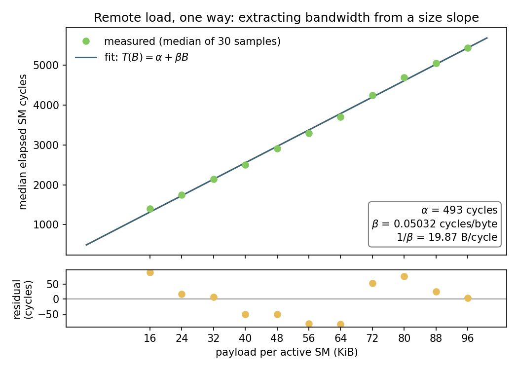
Remote load, one way, used here as the worked example. The top panel plots
median elapsed SM cycles against payload per active SM, with the affine fit
overlaid; alpha is a combined fill/drain and completion term, not a
separately measured hardware latency, while 1/beta is the sustained
bandwidth. The bottom panel plots the residual cycles around zero.
Baseline DSM Bandwidth
The first result is that all three data-movement mechanisms converge near 20 bytes per SM cycle:
| operation | one-way B/cycle | one-way GB/s |
|---|---|---|
| remote load | 19.87 | 35.83 |
| ordinary remote store | 18.87 | 33.68 |
| TMA remote put | 21.25 | 37.90 |
This number looked strange. I expected something related to a 32-B/cycle SM interface, but 20–21 B/cycle is neither 32 B/cycle nor an obvious half-width 16 B/cycle interface.
One possible explanation was that the DSM fabric runs in a separate clock domain around 1 GHz. The two timers make that unnecessary. The ratio between the fitted cycle slope and nanosecond slope stays near 1.77–1.80 cycles/ns, consistent with the approximately 1.785-GHz maximum SM clock reported during the run. There may still be a clock-domain crossing inside the implementation, but the observed bandwidth does not require one to explain the number.
Bidirectional Reads Lose Bandwidth, but Writes Almost Do Not
The more interesting result appears when SM0 and SM1 access each other at the same time. A symmetric read drops from 19.87 to 15.37 B/cycle per direction, losing 22.6% of its bandwidth. In contrast, normal stores drop only from 18.87 to 18.12 B/cycle, and TMA puts from 21.25 to 20.29 B/cycle. Both retain 94–96% of their one-way rate.
Honestly, the write result was more surprising than the read result. A single universal half-duplex port would penalize all three operations. A TMA-only shortcut also cannot explain the result, because an ordinary store can write remote shared memory and shows the same duplex behavior.
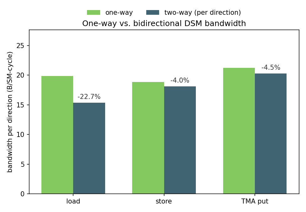
Fitted bandwidth per direction for load, store, and TMA put, one-way versus bidirectional. Symmetric reads lose 22.7% per direction, while symmetric stores and TMA puts lose only 4.0% and 4.5%. Aggregate two-way bandwidth is not shown, since it would hide the per-direction loss discussed here.
Mixed Traffic Finds the Shared Directional Resource
To determine whether read responses and write data use the same resource, I run two payloads at once. Rank 0 always reads rank 1, so read-response data travels from rank 1 to rank 0. A normal store or TMA put carries a second payload either in the same physical data direction or in the opposite direction.
When both payloads travel in the same direction, their aggregate rate collapses to the same approximately 21-B/cycle ceiling: 21.38 B/cycle for load plus store and 21.45 B/cycle for load plus TMA put. Reversing the write payload raises them to 29.70 and 29.26 B/cycle, respectively, an increase of 37–39%.
This experiment is useful because it separates instruction front ends from the network direction. Normal store and TMA agree within about 1%, so their shared limit is downstream of the issuing instruction. Read-response data and write payload data share a directional physical resource, even if the protocol places them in different logical queues or virtual channels.
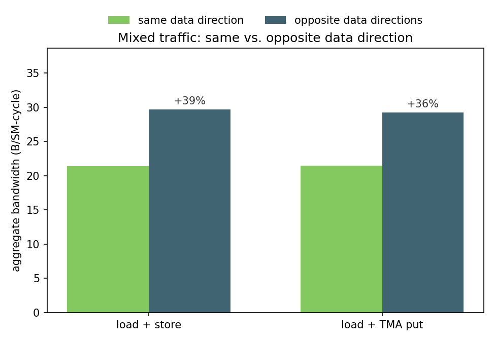
Aggregate B/SM-cycle when rank 0’s read response and the second payload (store or TMA put) share the same physical direction versus opposite directions. Reversing the write payload increases aggregate throughput by 39% and 36%, showing that read-response data and write payload data share a directional physical resource.
What NVIDIA’s Patent Tells Us
At this point the measurements constrain directionality, but not the physical structure. The most useful public description I found is NVIDIA’s US12248788B2, Distributed shared memory, especially Figures 21A–21D.
TPCARB first arbitrates traffic from SMs in the same TPC. For DSM routing,
the uTLB performs address hashing rather than ordinary virtual-to-physical
translation, distributing requests across GXBAR paths to avoid camping.
GPCARB then routes SM-to-SM traffic through GXBAR and, on the destination
side, fans it out to the target SM.
Figure 21A locates the physical convergence more precisely. The connection
from GPCMMU to GPCARB ingress is explicitly labeled 6 mmu2gpcarb: the six SM
paths are still distinct after TPCARB and GPCMMU. Only the output of GPCARB
ingress is labeled SM2SM4. The structural narrow waist is therefore not in
GPCMMU; it is the six-input/four-output GPCARB ingress and its four-lane
interface to GXBAR.
This does not require repacking a flit. If an input and an output lane both carry 32 B, GPCARB simply selects up to four of six ready input flits each cycle. Multi-flit packets remain sequences of same-width flits.
Ingress and Egress Are Organized Differently
Figure 21B’s port assignments are asymmetric between ingress and egress, and that asymmetry turns out to matter. The mapping is visible directly in Patent Figure 21B.
At ingress, each CPC’s six source SMs feed one GPCARB-IG, which gets two
ports on GX0 and two on GX1. That gives four lanes per CPC and twelve
GPC-wide, matching the SM2SM4/SM2SM12 names. GX0 and GX1 are separate
6×6 switch planes, not one ordinary 12×12 crossbar.
Egress is organized differently. Each CPC has two GPCARB-EG blocks; each EG
takes one output from GX0 and one from GX1, then fans out to three destination
SMs. The destination side therefore still has four aggregate lanes per CPC,
but they are split into two independent two-lane, three-SM groups. The figure
below carries the detailed IG, GX, and EG port mapping.
This also gives a cleaner reading of why adjacent SM pairs looked fast in the
topology sweep. If two adjacent SMs correspond to the two SM slots of the
same TPC, they land on different EGs (SM0 on EG0, SM1 on EG1), so a
bidirectional exchange between them can use two different EGs, two different
GX output ports, and both GX planes simultaneously – without requiring any
TPC-local bypass of GXBAR. I want to flag a real limit here, though: the
patent’s figure uses 18 logical SM slots with its own floorsweeping, and my
CUDA cluster ranks are not guaranteed to line up with that SM0…SM17
numbering. This mapping is useful for a simulator, but I cannot claim that a
measured %smid parity bit is literally the EG-select bit.
This is one layer more specific than “six SMs share four lanes”: the four lanes are contended as a single pool at ingress, but organized as two independent two-lane, three-SM fan-out groups at egress.
For a source CPC talking to one destination EG, there are four structurally
distinct routes: GX0’s two candidate inputs and GX1’s two candidate inputs
each reach that EG’s one output on their respective plane. The uTLB address
hash most likely selects among these four equivalent routes to spread load
and avoid camping – which is also four, matching the four SM2SM4 lanes.
Three CPC SM2SM4 paths are combined into the GPC-level SM2SM12 network.
These names describe aggregate connections, not a one-to-one mapping between
network ports and the 16 CUDA cluster ranks used in my experiment.
GX0 and GX1 are parallel switch planes or paths. They are not the request and response virtual channels. The patent says firmware may shut down one plane and retain connectivity at reduced bandwidth. An address selects a route through GXBAR, and a request and its response may use different internal paths.
Every packet generated by an SM uses the outgoing path through TPCARB,
GPCMMU, GPCARB ingress, and GXBAR, whether it is the original request or a
read response/write ACK generated by the target. The fold path for a
response does not need normal address translation, but Figure 21D still routes
the outgoing response through the uTLB/GPCMMU block. In contrast, an arriving
packet goes from GPCARB egress through the mapped request-or-response interface
directly to the SM; it does not revisit GPCMMU.
Thus a complete remote load uses the source GPCMMU when the request is sent and the target GPCMMU/fold path when the read response is sent. The request’s arrival at the target and the response’s arrival back at the source both go directly from GPCARB egress to the SM. A write ACK follows the same outgoing response path as read data, but carries much less information and can be coalesced.
The packet table is also revealing. Read commands use a blocking request VC, while read data and write acknowledgments use a non-blocking response VC. Read responses may contain one or multiple packets. Short writes include payload in the request packet, while long writes use a command followed by write-data packets.
Most importantly for the duplex result, write acknowledgments can be coalesced. A destination SM may count how many acknowledgments it owes each source and return an accumulated count when a threshold is reached or the bus is idle. A read cannot do the same thing with its response data.
The patent explicitly permits a bandwidth control that restricts how much data each SM may transfer per clock. It also describes outstanding transaction counters and address-based routing. However, it does not disclose the physical flit width, exact limiter placement or implementation, header encoding, arbitration schedule, fabric clock, address-hash function, or link-credit depth. I treat the topology and packet classes as patent facts; the numerical model below remains an inference from measurement.
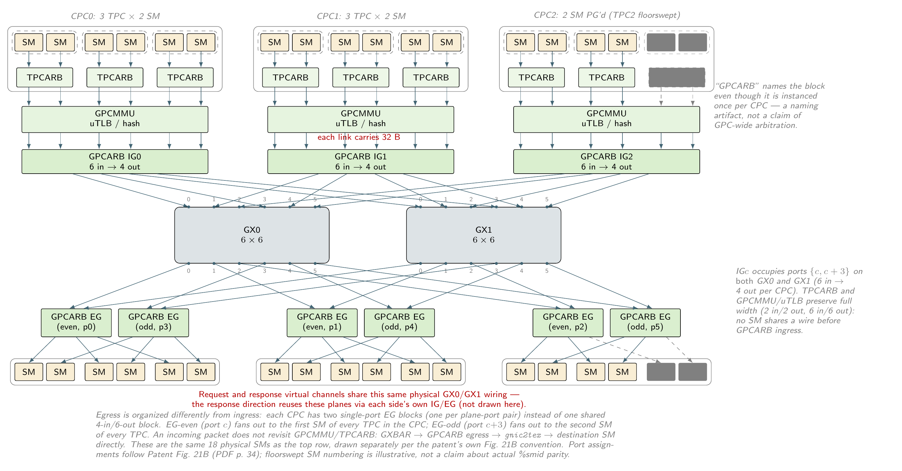
Source-to-destination DSM path, redrawn from Patent Figures 21A–21D. The diagram shows the 3 CPC × 3 TPC × 2 SM hierarchy, the six-to-four convergence at GPCARB ingress, the two 6×6 GX planes, and the asymmetric GPCARB egress.
A 32-Byte Lane with a 2/3 Per-SM Allocation
The SM2SM4 structure gives a simple back-of-the-envelope explanation for the
otherwise strange 21-B/cycle result. Suppose each aggregate lane carries 32 B
per cycle. Four lanes shared equally by six SM clients provide
This independently matches one-way load, normal store, TMA put, and multi-SM TMA scaling. The physical four-lane convergence alone does not explain why one SM cannot use an otherwise idle 32-B lane. The measurements point to the per-SM bandwidth control mentioned by the patent being configured as a hard limiter near the SM-facing injection path:
- one active SM reaches only about 20–21 B/cycle even when the rest of the CPC is idle;
- two active SMs each remain near 21 B/cycle rather than reclaiming unused CPC capacity;
- 2/4/8/16-SM TMA slopes stay near the same rate per SM;
- cold-burst and gap tests reveal no material temporary rate above the steady limit.
My working model is therefore that the SM injection path itself is shaped to
4/6 of one nominal 32-B lane. The shaper prevents the six inputs from
offering more than four lanes in aggregate, while GPCARB ingress is where those
six still-distinct physical paths actually converge onto SM2SM4. The exact
limiter circuit may be inside the SM request interface or immediately beside
it; the patent does not draw that boundary. What matters for the model is that
the allocation is hard and non-work-conserving, rather than fairness emerging
only after six unrestricted SMs contend at GPCARB.
Why Bidirectional Reads Lose About One Quarter
The remaining question is why symmetric reads fall from 19.87 to 15.37 B/cycle per direction.
A plausible saturated read-response quantum is 128 B, transported as four 32-B flits. With six clients sharing four lanes, one 32-B flit costs an average of
$$ \frac{6}{4}=1.5\ \mathrm{SM\ cycles}. $$For a one-way read response:
$$ 4\ \mathrm{response\ flits}\times1.5=6\ \mathrm{cycles}, $$so
$$ \frac{128\ \mathrm{B}}{6\ \mathrm{cycles}} =21.333\ \mathrm{B/cycle}. $$During symmetric reads, each directional allocation carries four response-data flits plus approximately one read-command flit requesting the response in the opposite direction:
$$ (4+1)\times1.5=7.5\ \mathrm{cycles}, $$giving
$$ \frac{128\ \mathrm{B}}{7.5\ \mathrm{cycles}} =17.067\ \mathrm{B/cycle}. $$The measured one-way load reaches 19.874 rather than the ideal 21.333 B/cycle. Applying that measured utilization to the ideal duplex prediction gives
$$ 17.067\times\frac{19.874}{21.333} =15.900\ \mathrm{B/cycle}. $$The measured result is 15.372 B/cycle, only 3.4% lower.
Another way to view the same data is cost per 128 B. Measurement increases from 6.441 cycles one way to 8.327 cycles two way. The extra 1.886 cycles is close to one shaped 32-B flit at 1.5 cycles, with the remaining difference plausibly coming from arbitration, trackers, credits, or metadata bubbles.
Other response sizes are less convincing under the same one-command-flit assumption:
| response data | data flits | ideal two-way rate | ideal duplex loss |
|---|---|---|---|
| 64 B | 2 | 14.22 B/cycle | 33.3% |
| 128 B | 4 | 17.07 B/cycle | 20.0% |
| 256 B | 8 | 18.96 B/cycle | 11.1% |
A warp-wide ld.shared::cluster.v4.b32 returns 512 useful bytes and can
naturally decompose into four 128-B shared-memory wavefronts. This makes 128 B
a plausible response/coalescing quantum. It does not mean there is a
128-byte physical wire.
Writes have a different packet composition. Their payload travels with the write request or in following write-data packets. The reverse direction needs only an acknowledgment, and the patent explicitly allows many acknowledgments to be combined. This naturally explains why two-way store and TMA traffic lose only 4–5% instead of the read path’s 23%.
Scaling from 2 to 16 SMs
The next test has every active SM use TMA to put one tile to its ring neighbor. I apply the same 16–96-KiB size-slope fit independently at 2, 4, 8, and 16 SMs:
| active SMs | aggregate B/cycle | aggregate GB/s | per-SM B/cycle |
|---|---|---|---|
| 2 | 40.59 | 72.86 | 20.29 |
| 4 | 82.02 | 145.06 | 20.50 |
| 8 | 164.30 | 292.00 | 20.54 |
| 16 | 338.89 | 606.00 | 21.18 |
The 16-SM result is within 0.72% of
$$ 16\times21.333=341.33\ \mathrm{B/cycle}. $$There is no visible shared GPC-level put-data saturation through 16 SMs. Even more importantly, the two-SM case remains close to 21 B/cycle per SM although most potential clients are idle. Spare service is not visibly reclaimed. This is why I prefer a fixed TDM-like allocation over a normal work-conserving crossbar model.
The size slope matters especially here. The fitted completion intercept grows from about 1,101 cycles at two SMs to about 5,256 cycles at 16 SMs, while the incremental slopes remain nearly equal. A single 64-KiB throughput point would mix this cluster-size-dependent completion cost into the network rate and make scaling look much worse than it is.
How Much Topology Can We Recover?
I next fix the payload at 64 KiB per active SM and compare traffic patterns of the same shape. These raw rates are useful for relative topology comparisons, not for extracting the steady physical bandwidth described above.
| topology | aggregate bandwidth |
|---|---|
| 2-SM ring | 51.2 GB/s |
| 4-SM ring | 102.4 GB/s |
| 8-SM ring | 204.8 GB/s |
| 16-SM ring | 344.9–372.4 GB/s, depending on stride |
| eight adjacent two-SM groups | 390.1 GB/s |
The 16-SM ring favors strides 2 and 14, reaching 372.4 and 368.2 GB/s, while several strides fall to 344.9 GB/s. Eight disjoint adjacent pairs are about 11% faster than the median 16-SM ring. This suggests a locality or arbitration boundary associated with the two-SM grouping.
However, isolated pairs reveal almost nothing. All 240 directed source/target pairs lie within 31.51–32.00 raw GB/s, and scanning a 32-B address offset over 4 KiB changes cycles by only 0.39%. Route hashing and camping become visible mainly when many flows contend simultaneously.
This is not enough information to recover NVIDIA’s exact address hash, and I am not sure doing so is particularly useful. A first simulator can use a simple deterministic cache-line or packet interleave that reproduces stride-dependent camping. The data also does not prove a special TPC-local bypass: the patent’s illustrated route still passes through GPCARB and GXBAR.
Hypotheses That Did Not Survive
Several explanations looked plausible at intermediate stages but did not fit all the experiments:
- A separate 1-GHz DSM clock. It can turn the GB/s number into an appealing
bus width, but the cycle/ns slope and
4 * 32 / 6model already explain the observation in the SM clock domain. - One universal half-duplex SM port. This predicts a large duplex penalty for writes, which is not observed.
- A 64-B physical flit. A 64-B response quantum can be made to fit one bandwidth ratio, but predicts too much symmetric-read loss under the common one-command-flit model. The patent’s short-write payload is also naturally smaller than a full cache line.
- A TMA-only bypass. Ordinary remote stores and TMA puts have almost the same directional contention and duplex efficiency.
- The destination SRAM or a simple LSU stall. Adding up to 16 warps of local shared-memory pressure, including a conflicting bank pattern, leaves remote-load completion essentially unchanged at 3,628–3,633 cycles.
- A large token bucket. Cold commands, command trains, and separated bursts do not reveal material temporary bandwidth above the approximately 21.3-B/cycle rate. A very small hidden bucket remains possible.
- A TPC-local DSM bypass. Adjacent pairing is favorable under concurrency, but neither the patent route nor isolated-pair latency/bandwidth provides evidence for bypassing the GPC-level path.
Virtual Channels, Credits, and Deadlock
The patent’s blocking request and non-blocking response VCs are useful for protocol separation, but virtual channels are logical queues multiplexed over physical links. They do not contradict the mixed-traffic directional ceiling.
Credits are also easy to over-interpret. A link credit normally represents free downstream buffer capacity and prevents overflow. It is not itself a fairness policy, and credits alone cannot break a cyclic channel dependency. Deadlock avoidance additionally needs restricted VC transitions, an acyclic dependency graph, or an escape VC.
The patent’s endpoint outstanding-transaction counters are a different level of accounting. They track whether loads have received all response data and whether stores have received accumulated acknowledgments, allowing barriers and CTA exit to wait for DSM operations to complete. The patent does not reveal the per-hop link-credit implementation.
Key Takeaway
The robust measurements are:
- one SM sustains about 20–21 B/cycle of DSM traffic;
- symmetric reads lose 22–23% per direction;
- symmetric normal stores and TMA puts lose only 4–6%;
- read responses and write payloads share a directional physical ceiling;
- TMA puts scale linearly from 2 to 16 SMs at about 21 B/SM-cycle;
- concurrent traffic reveals a favorable adjacent two-SM grouping and stride-dependent contention.
The strongest model consistent with those results is:
- four 32-B lanes serve six SM clients in each CPC;
- each SM sees a non-work-conserving
2/3-lane allocation; - request and response virtual queues share directional lane service;
- saturated reads likely use a 128-B response quantum plus an opposite read command;
- writes carry payload forward and amortize reverse traffic through coalesced acknowledgments.
I do not claim that the model is bit accurate. Literal TDM versus an equivalent issue shaper, exact packet headers, address hashing, link-credit depth, and any internal clock-domain crossing remain unresolved. But the model explains every robust bandwidth result with one fairly small set of assumptions, and it is simple enough to use in a first-order simulator.