Understanding Transformer Decoder
I have been extremly late to the party of transformer, and here is my note on understanding the flops, data movements, compute intensity, etc.
Note: For simplicity, I omit the data type for now.
Decoder-Only Transformer
Let’s start with something simple: a decoder-only transformer. Also, we skip the initial step to map token into the dictionary space with positionary encoding. If we look at a single layer of the decoder architecture, it contains three parameters:
- Batch size \(B\)
- Sequence length \(S\)
- Hidden dimension \(D\)
For the forward pass, it contains the following stages:
Scaled Dot-Product Attention
First, we compute the QKV matrix from linear transformation of the input:
- Input (from positionary encoding or previous layer): \([BS, D]\)
- Weight: Each Q/K/V matrix requires \([D, D]\) weight
- Output: Q/K/V matrix each of size \([BS, D]\)
- Flop (three matrix Q/K/V): \(3\times2BSDD=6BSD^2\)
- Data Read: \((BSD + 3D^2)\)
- Data Write: \(3BSD\)
Then we apply the attention:
\(\mathrm{Attention}(Q,K,V)=\mathrm{softmax}(\frac{QK^{T}}{\sqrt{D}})V\)
This involves two matrix multiplication: \(QK^T\) and finally multiply with \(V\).
For \(QK^T\):
- Input: \(Q=[S, D]\), \(K^T=[D, S]\)
- Output: \(A=[S, S]\)
- Flop (notice the batch size \(B\)): \(2BS^2D\)
- Data Read: \(2BSD\)
- Data Write: \(BS^2\)
For multiplication with \(V\):
- Input: \(A=[S, S]\), \(V=[S, D]\)
- Output: \(O=[S, D]\)
- Flop (notice the batch size \(B\)): \(2BS^2D\)
- Data Read: \((BS^2 + BSD)\)
- Data Write: \(BSD\)
FFN
This usually first uses \(W_1\) to project \(x\) to some higher dimensions \(D_{up}\), applies an activation function, then projects down to the original hidden space.
\(\mathrm{FFN}(x) = \mathrm{Activation}(xW_1+b_1)W_2+b_2\)
The activation function can be simple as ReLU, or more complicated
ones involving more matrix multiplication (see below for the case
study of Llama). Here we assume the activation function does not
introduce more tensor operation.
For up projection:
- Input: \([S, D]\), \([D, D_{up}]\)
- Output: \(A=[S, D_{up}]\)
- Flop (notice the batch size \(B\)): \(2BSDD_{up}\)
- Data Read: \((BSD + DD_{up})\)
- Data Write: \(BSD_{up}\)
For down projection:
- Input: \([S, D_{up}]\), \([D_{up}, D]\)
- Output: \(A=[S, D]\)
- Flop (notice the batch size \(B\)): \(2BSDD_{up}\)
- Data Read: \((BSD_{up} + DD_{up})\)
- Data Write: \(BSD\)
Note: These stages make the backbone of transformer.
Multi-Head Attention (MHA)
Now we move on to some variants. We can also replace the scaled dot-product attention with multi-head attention, which essentially requires breaking the attention into \(N\) heads, each with lower dimensions \(D_h\) and with \(D=ND_h\):
\(\mathrm{MultiHead}(Q,K,V)=\mathrm{Concat}(head_i)W_o\)
Where each head is an output of the attention:
\(head_i=\mathrm{Attention}(QW_{Qi}, KW_{Ki}, VW_{Vi})\)
Here each \(W_i\) is learned parameters. Since \(Q\), \(K\), \(V\) are also learned linear transformation from the embedding, we can immediately fuse those two weight together:
\(Q_i=QW_{Qi}=Input\times W_Q\times W_{Qi}=Input\times W'_{Qi}\)
Hence, the QKV generation stays the same.
Therefore, for all heads (reusing prior attention results):
- Input: \(Q_i=[S, D_h]\), \(K_i^T=[D_h, S]\)
- Output: \(A_i=[S, S]\)
- Flop (notice the batch size \(B\) and heads num \(N\)): \(4BNS^2D_h=4BS^2D\)
Note: breaking the attention into multiple heads does not save computation, but simply allows each head focus on different representation subspace.
The final output weight:
- Input: \([S, D]\), \([D, D]\)
- Output: \(O=[S, D]\)
- Flop (notice the batch size \(B\)): \(2BSD^2\)
Group Query Attention (GQA)
In order to save some storage and computation, group query attention (GQA) groups attention heads into \(G\) groups. Heads within the same group share the key and value. Therefore, it saves the memory space for the K-V cache (see below) and the computation to generate the key/value.
The Q matrix is generated the same as in MHA. However, there is only \(G\) keys and values:
- Compute Flop: Q: \(2BS(ND_h)^2\), K/V: \(4BSNGD_h^2\)
The original K/V is of size \([B, S, G, D_h]\), and we will repeat by \(N/G\) times and make it the same as \([B, S, N, D_h]\) for normal MHA.
Note: GQA saves computation on generating key and value, and memory space on caching key and value.
Swish-GLU FFN
Another commonly used variant of FFN is using Swish-GLU for the activation function. The overall formula is:
\(\mathrm{FFN}(x) = \mathrm{Swish\text-GLU}(xW_1+b_1)W_2+b_2\)
\(\mathrm{Swish\text-GLU}(x)=(xW_3+b_1)\cdot\sigma(\beta(xW_4+b_4))\)
Usually we have \(\beta=1\) and all bias \(b_i\) to zero. Then the formula can be simplified as:
\(\mathrm{FFN}(x) = ((xW_1W_3)\cdot\sigma(xW_1W_4))W_2\)
Clearly this can be simplified into three weights:
- \(W'_1=W_1W_3=[D, D_{up}]\)
- \(W'_2=W_1W_4=[D, D_{up}]\)
- \(W'_3=W_2=[D_{up}, D]\)
Rotary Position Embedding (RoPE)
So far all the computation is independent to the position of the token in the sequence, since QKV are just linear projection of the embedding. However, the relative location between two tokens are important for reasoning, e.g. “do I” is different than “I do”. Rotary Position Embedding (RoPE) is used to add back the position information to the embedding. The formula is quite simple:
\(\mathrm{RoPE}(pos, j)=e^{i \frac{pos}{\lambda}},\lambda=\theta^{j/D_h}\)
Quote from the classic Attention is all you need:
That is, each dimension of the positional encoding corresponds to a sinusoid. The wavelengths form a geometric progression from 2π to 10000 2π. We chose this function because we hypothesized it would allow the model to easily learn to attend by relative positions, since for any fixed offset k, PE(pos+k) can be represented as a linear function of PE(pos).
When transforming, each attention head’s key and query is grouped by
2 to form a complex number, and then rotate by RoPE.
Note: RoPE does not invole matrix multiplication nor parameters.
Case Study on Llama3-70B
We have almost everything together to understand the architecture of Llama3-70B. Here is a handy simple implmenation llama3 and the parameters here:
{
  "architectures": [
    "LlamaForCausalLM"
  ],
  "attention_bias": false,
  "attention_dropout": 0.0,
  "bos_token_id": 128000,
  "eos_token_id": 128001,
  "hidden_act": "silu",
  "hidden_size": 8192,
  "initializer_range": 0.02,
  "intermediate_size": 28672,
  "max_position_embeddings": 8192,
  "model_type": "llama",
  "num_attention_heads": 64,
  "num_hidden_layers": 80,
  "num_key_value_heads": 8,
  "pretraining_tp": 1,
  "rms_norm_eps": 1e-05,
  "rope_scaling": null,
  "rope_theta": 500000.0,
  "tie_word_embeddings": false,
  "torch_dtype": "bfloat16",
  "transformers_version": "4.40.0.dev0",
  "use_cache": true,
  "vocab_size": 128256
}
First of all, llama3 uses GQA and Swish-GLU FFN. Let’s see if we can understand these numbers:
- Hidden dimension \(D=8192\)
- Head number \(N=64\) (which is
num_attention_heads) - Group number \(G=8\) (which is
num_key_value_heads) - Head dimension \(D_h=D/N=128\)
- FFN up dimension \(D_{up}=4D=32768\)
- Hidden layers \(L=80\)
Model Size (Weights)
| Stage | Weight Dim | Num Elem | Tensor Flop | Tensor Flop |
|---|---|---|---|---|
| Generate Q | \([D, D_hN]\) | 64Mi | \(2SD^2\) | 1T |
| Generate K | \([D, D_hG]\) | 8Mi | \(2SDD_hG\) | 128M |
| Generate V | \([D, D_hG]\) | 8Mi | \(2SDD_hG\) | 128M |
| Attention Out | \([D, D]\) | 64Mi | \(2SD^2\) | 1T |
| Swish-GLU FFN \(W_1\) | \([D, D_{up}]\) | 256Mi | \(2SDD_{up}\) | 4T |
| Swish-GLU FFN \(W_2\) | \([D, D_{up}]\) | 256Mi | \(2SDD_{up}\) | 4T |
| Swish-GLU FFN \(W_3\) | \([D_{up}, D]\) | 256Mi | \(2SDD_{up}\) | 4T |
| One Layer | 912Mi | 14.25T | ||
| All | 72960Mi | 1140T |
Since \(72960Mi\approx 76\times 10^9=76B\), we now know
why it is called llama3-70B.
- Takeaway 1: The FFN is still the most compute-intensive part.
- Takeaway 2: The model is so large that a single GPU does not come with sufficient memory to hold it.
- Takeaway 3: A RTX 4090 comes with 512 tensor cores, each can perform 1024 FP Flop per cycle, and boost frequency 2.52GHz – peak compute throughput is 1.32PFlops – and it still takes about ~0.86s to finish all these computation. LLM is expensive!
To Summarize:
| Stage | Matrix Flop | Read | Write |
|---|---|---|---|
| QKV | \(6\times BS(ND)^2\) | ||
| Multi-Head Atten. | \(2\times BSND(2S+ND)\) | ||
| FFN | \(4\times BSN^2DD_{up}\) |
For example: when \(B=4,S=4096,N=1,D=128, D_{up}=512\), we have:
- QKV: 1.5 GFlop
- Multi-Head Attention: 32.5 GFlop
- FFN: 4 GFlop
Total we have 38 GFlop, if we have a 1.7 PFlops device, the tensor core busy time would be \(38/1.7=22.3\mathrm{us}\)
K-V Cache and Inference
As we have seen, during inference, we compute each token’s query with all prior tokens’ key for a score, and then use that score to accumulate all prior tokens’ value. The inference can be further broken into two steps:
- Prefill: This part feeds the entire user prompt to the model. This sets up the context for the model, and is why there is some waiting time before ehe first word popping on your screen.
- Decode: Once the context is set up, self-regressive decoding starts – each step the model generates one token, and appends that token to the context (extending the sequence length by 1).
As you can imagine, during decode step, the key/value of all prior tokens do not change, and if we can save it in a cache (hence the name K-V cache), we could save the computation on computing \(K\) and \(V\). Hence, since \(S=1\) in decode step, it is GEMV and therefore usually memory bounded on streaming the weight and key/values.
DeepSeek-V3
DeepSeek-V3 is phenomenal these days, and here are my notes trying to understanding these topics:
- Multi-Head Latent Attention (MLA)
- Mixture-of-Experts (MoE)
Multi-Head Latent Attention (MLA)
K-V Cache is Huge
The K-V cache significantly reduces the computation for attention, but at the cost of exploding storage of the context. For every context:
\(\mathrm{KVElem}(L,S,D)=2LSD\)
Obviously, this limits the number of concurrent users the system can support, as well as the context length. For example, the above llama3 would take \(2\times80\times8k\times8k\times2B=20\mathrm{GB}\) for one 8k context. For reference, a 4090 only has 24GB graphic memory.
Compress Key/Value
To save the space on key-value cache, DeepSeek-V2 introduces multi-head latent attention (MLA). The idea is fairly simple – compress the key-value into some latent space with lower dimension and cache it.When computing, project it back for normal attention computation.
Down-project:
\(c^{KV}=W^{DKV}h\)
Up-project:
\(k^C=[k^C_0,...,k^C_{N_C}]=W^{UK}c^{KV}\)
\(v^C=[v^C_0,...,v^C_{N_C}]=W^{UV}c^{KV}\)
Note: The key and value are jointly compressed.
Compress Query
We can also do the same on the query \(q\). This does not save us anything during inference since \(q\) is not cached, but it does help save the space during training.
\[ c^{Q}=W^{DQ}h \]\[ q^C=[q^C_0,...,q^C_{N_C}]=W^{UQ}c^{Q} \]Decoupled RoPE
If you remember, we apply RoPE on \(q\) and \(k\) to encode the position information, and normally we save \(k\) after we applied RoPE to the K-V cache. However, since we jointly compress \(k\) and \(v\) into \(c^{KV}\), and \(v\) is independent of the position, we can not encode the position information into \(c^{KV}\). On the other hand, we definitely don’t want to apply RoPE on \(k^C\), as that’s of complexity \(BSD^2\) and a waste of computation.
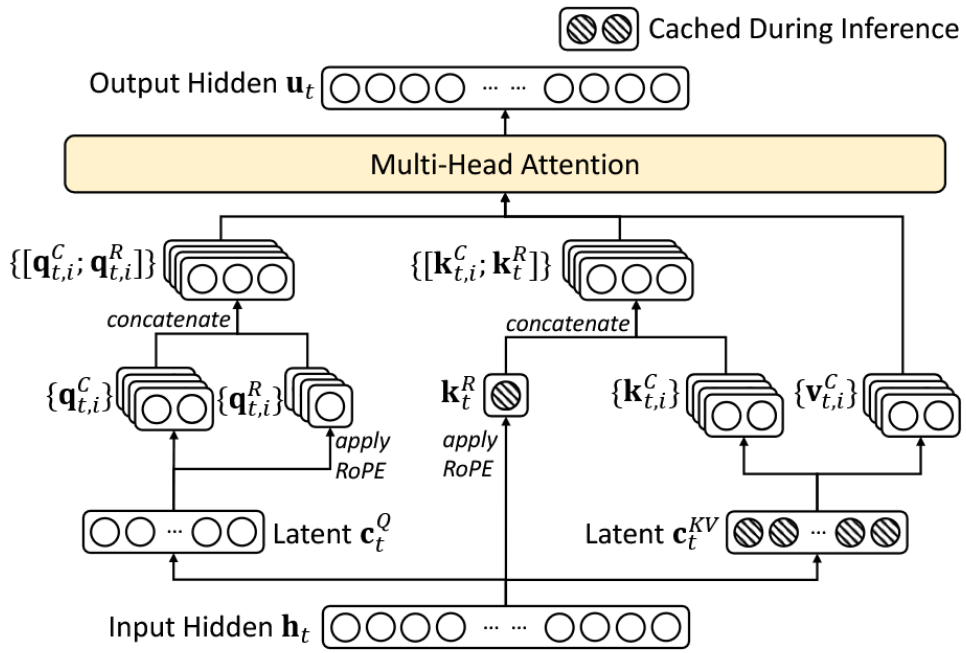
Therefore, the authors introduce decoupled RoPE – basically two sets of heads, one apply RoPE and the other don’t (with superscript \(R\) for rotary and the above superscript \(C\) for constant), then we simply concatenate \(q=[q^C,q^R]\) and \(k=[k^C,k^R]\) for attention.
\[ q^R=[q^R_0,...,q^R_{N_R}]=\mathrm{RoPE}(W^{QR}c^{Q}) \]\[ k^R=[k^R_0,...,k^R_{N_R}]=\mathrm{RoPE}(W^{KR}h) \]
Put Everything Together
Below is the figure showing the overal MLA architecture. Note that only \(c^{KV}\) and \(k^R\) is cached. You can also find the implementation here.
Let’s try to implement this in pytorch style code with detailed comment:
def MLA(hidden_state):
  # Compute the compressed query c_q, c_kv, k_r together
  # [b, s, d] * [d, q_lora_rank + kv_lora_rank + d_r] -> [b, s, q_lora_rank + kv_lora_rank + d_r]
  x = torch.matmul(hidden_state, W_DQ_DKV_KR)

  ############### FA Pre ####################
  # Up project. Notice that we can combine q_c and q_r together
  c_q = x[..., :q_lora_rank]
  c_q = rmsnorm(c_q)
  # [b, s, q_lora_rank] * [q_lora_rank, n * (d_c + d_r)] -> [b, s, n * (d_c, d_r)]
  q = torch.matmul(c_q, W_UQ_QR)

  # Group q by attention heads and split into q_c and q_ra
  q = q.view(b, s, n, (d_c + d_r)).transpose(1, 2) # [b, n, s, d_c + d_r]

  # Apply RoPE to q_r and regroup into q.
  q_r = q[..., dc:]
  q_r = rope(q_r) # [b, n, s, d_r]

  # Apply RMS norm to c_kv.
  c_kv = x[..., q_lora_rank:q_lora_rank + kv_lora_rank]
  c_kv = rmsnorm(c_kv) # [b, s, kv_lora_rank]

  # Apply RoPE to k_r
  k_r = x[..., q_lora_rank + kv_lora_rank:]
  k_r = rope(k_r) # [b, s, d_r]

  # Update the KV-cache with compressed c_kv and k_r -- a vew of x
  end_pos = start_pos + s
  kv_cache[:b, start_pos:end_pos, :] = x[..., q_lora_rank:]

  # Compute the nope head score q_c * k_c^T = q_c * (c_kv * W_UK)^T = q_c * W_UK^T * c_kv^T
  q_c = q[..., :dc] # [b, n, s, d_c]
  # [b, n, s, d_c] * [n, d_c, kv_lora_rank] -> [b, n, s, kv_lora_rank]
  q_c = torch.matmul(q_c, W_UK_T)
  q = cat(q_c, q_r) # [b, n, s, kv_lora_rank + d_r]

  ############### FA ########################
  # Note this is batch GEMM with one to n query (similar to MQA)
  # [b, n, s, kv_lora_rank + d_r] * [b, 1, kv_lora_rank + d_r, end_pos] -> [b, n, s, end_pos]
  score = torch.matmul(score_c, kv_cache[:b, :end_pos, :].transpose(1, 2).unsqueeze(1))

  # Compute the softmax.
  score = (score + softmax_scale).softmax(dim=-1) # [b, n, s, end_pos]

  # Compute the value: score * v = score * (c_kv * W_UV)
  # [b, n, s, end_pos] * [b, 1, end_pos, kv_lora_rank] -> [b, n, s, kv_lora_rank]
  output = torch.matmul(score, kv_cache[:b, :end_pos, :kv_lora_rank].unsqueeze(1))

  ############### FA Post ###################
  # [b, n, s, kv_lora_rank] * [n, kv_lora_rank, d_v] -> [b, n, s, d_v]
  output = torch.matmul(output, W_UV)
  output = output.transpose(1, 2) # [b, s, n, d_v]

  # Final output.
  output = output.flatten(2) # [b, s, n, d_v] -> [b, s, n * d_v]
  # [b, s, n * d_v] * [n * d_v, d] -> [b, s, d]
  output = torch.matmul(output, W_O)